ШЋЮФЯТдиСДНгЃКhttp://tecdat.cn/?p=18266
БОЮФЭЈЙ§RгябдНЈСЂЙувхЯпадФЃаЭ(GLM)ЁЂЖрЯюЪНЛиЙщКЭЙувхПЩМгФЃаЭЃЈGAMЃЉРДдЄВтЫдк1912ФъЕФЬЉЬЙФсПЫКХГСУЛжаавДцЯТРДЁЃ
ЭиЖЫИУЪгЦЕКХЖЏЬЌВЛПЩв§гУstr(titanic)
Ъ§ОнБфСПЮЊЃК
SurvivedЃКГЫПЭДцЛюжИБъЃЈШчЙћДцЛюдђЮЊ1ЃЉPclassЃКТУПЭВеЮЛЕШМЖSexЃКГЫПЭадБ№AgeЃКГЫПЭФъСфSibSpЃКажЕмНуУУ/ХфХМШЫЪ§ParchЃКИИФИ/згХЎШЫЪ§EmbarkedЃКЕЧДЌИлПкNameЃКТУПЭаеУћ
зюКѓвЛИіБфСПЪЙгУВЛЖрЃЌвђДЫЮвУЧНЋЦфЩОГ§ЃЌ
titanic = titanic[,1:7]
ЯждкЃЌЮвУЧЛиД№ЮЪЬтЃК
авДцЕФТУПЭБШР§ЪЧЖрЩйЃП
МђЕЅЕФД№АИЪЧ
mean(titanic$Survived)[1] 0.3838384
ПЩвддкЯТУцЕФСаСЊБэжаевЕН
table(titanic$Survived)/nrow(titanic)0 10.6161616 0.3838384
ЛђДЫДІавДцепЕФ38.38 ЃЅЁЃвВОЭЪЧЫЕЃЌвВПЩвдЭЈЙ§ВЛЖдШЮКЮНтЪЭБфСПНјааТпМЛиЙщРДЛёЕУЃЈЛЛОфЛАЫЕЃЌНіЖдГЃЪ§НјааЛиЙщЃЉЁЃЛиЙщИјГіСЫЃК
Coefficients:(Intercept)-0.4733
Degrees of Freedom: 890 Total (i.e. Null);  890 ResidualNull Deviance:      1187Residual Deviance: 1187   AIC: 1189
ИјГіІТ0ЕФжЕЃЌВЂЧвгЩгкЩњДцИХТЪЮЊ 
ЮвУЧЭЈЙ§ПМТЧ 
exp(-0.4733)/(1+exp(-0.4733))[1] 0.3838355
ЮвУЧвВПЩвдЪЙгУpredictКЏЪ§
predict(glm(Survived~1, family=binomial,type="response")[1]10.3838384
ДЫЭтЃЌдкИХТЪЛиЙщжавВЪЪгУЃЌ
reg=glm(Survived~1, family=binomial(link="probit"),data=titanic)predict(reg,type="response")[1]10.3838384
авДцЕФЭЗЕШВеГЫПЭЕФБШР§ЪЧЖрЩйЃП
ЮвУЧжЛПДЭЗЕШВеЕФШЫЃЌ
[1] 0.6296296
дМ63ЃЅДцЛюЁЃЮвУЧПЩвдНјааТпМЛиЙщ
Coefficients:(Intercept)      Pclass2      Pclass30.5306      -0.6394      -1.6704
Degrees of Freedom: 890 Total (i.e. Null);  888 ResidualNull Deviance:      1187Residual Deviance: 1083   AIC: 1089
гЩгкЕк1РрЪЧВЮПМРрЃЌвђДЫЮвУЧееОЩПМТЧ 
exp(0.5306)/(1+exp(0.5306))[1] 0.629623
predictдЄВт
predict(reg,newdata=data.frame(Pclass="1"),type="response")10.6296296
ЮвУЧПЩвдГЂЪдИХТЪЛиЙщЃЌЮвУЧЕУЕНЕФНсЙћЪЧвЛбљЕФЃЌ
predict(reg,newdata=data.frame(Pclass="1"),type="response")10.6296296
ПЈЗНЖРСЂадВтЪд ЃКдкЩњДцгыЗёжЎМфЕФМьбщЭГМЦСПЪЧЖрЩйЃП
ПЈЗНМьбщЕФУќСюШчЯТ
chisq.test(table( Survived, Pclass))
Pearson's Chi-squared test
data:  table( Survived,  Pclass)X-squared = 102.89, df = 2, p-value < 2.2e-16
ЮвУЧгавЛИіСаСЊБэЃЌШчЙћБфСПЪЧЖРСЂЕФЃЌЮвУЧга  ЃЌШЛКѓЪЧЭГМЦСП
  ЃЌЮвУЧПЩвдПДЕНЃЌЖдВтЪдЕФЙБЯз
1.
1 2 30 -4.601993 -1.537771 3.9937031 5.830678 1.948340 -5.059981
етИјСЫЮвУЧКмЖраХЯЂЃКЮвУЧЙлВьЕНСНИіе§жЕЃЌЗжБ№ЖдгІгкЁАавДцЁБКЭЁАЭЗЕШВеЁБгыЁАЮоЗЈавДцЁБКЭЁАШ§ЕШВеЁБжЎМфЕФЧПЃЈе§ЃЉЙиСЊЃЌвдМАСНИіКмЧПЕФИКжЕЃЌЖдгІгкЁАЩњДцЁБКЭЁАЕкШ§ЕШЁБжЎМфЕФЧПСвИКЯрЙиЃЌвдМАЁАЮоЗЈавДцЁБКЭЁАЭЗЕШВеЁБЁЃЮвУЧПЩвддкЯТЭМЩЯПЩЪгЛЏетаЉжЕ
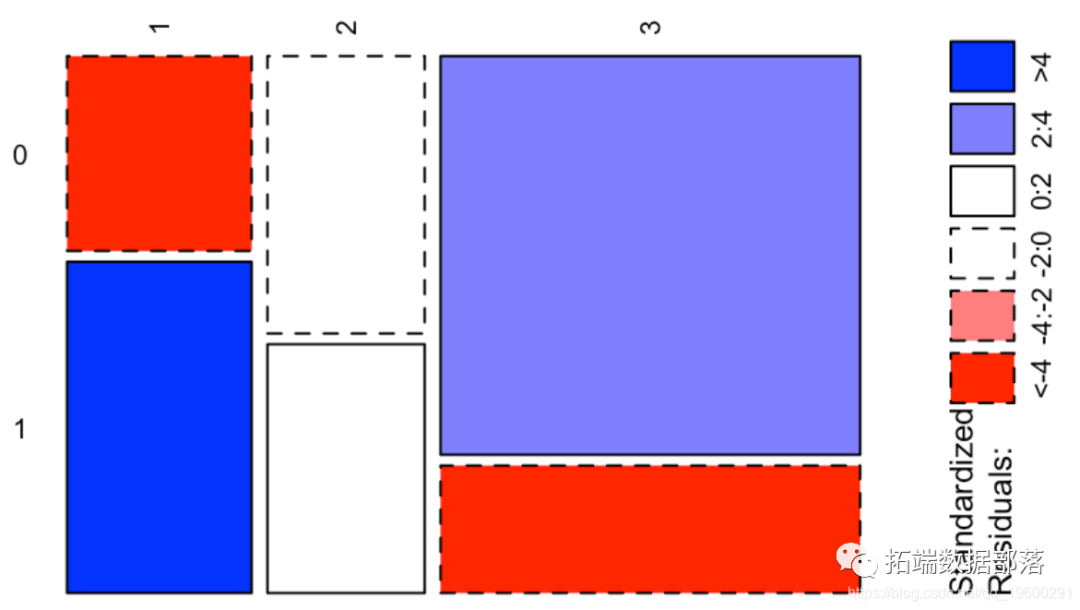
ass(table( Survived, Pclass), shade = TRUE, las=3)

ШЛКѓЮвУЧБиаыНјааТпМЛиЙщЃЌВЂдЄВтСНУћФЃФтГЫПЭЕФЩњДцИХТЪ
ЕуЛїБъЬтВщдФЭљЦкФкШн

RгябдБДвЖЫЙЙувхЯпадЛьКЯЃЈЖрВуДЮ/ЫЎЦН/ЧЖЬзЃЉФЃаЭGLMMЁЂТпМЛиЙщЗжЮіНЬг§СєМЖгАЯьвђЫиЪ§Он
01

02

03
04

МйЩшЮвУЧгаСНУћГЫПЭ
newbase = data.frame(Pclass = as.factor(c(1,3)),Sex = as.factor(c("female","male")),Age = c(17,20),SibSp = c(1,0),Parch = c(2,0),
ШУЮвУЧЖдЫљгаБфСПНјааМђЕЅЛиЙщЃЌ
Coefficients:Estimate Std. Error z value Pr(>|z|)(Intercept) 16.830381 607.655774 0.028 0.97790Pclass2 -1.268362 0.298428 -4.250 2.14e-05 ***Pclass3 -2.493756 0.296219 -8.419 < 2e-16 ***Sexmale -2.641145 0.222801 -11.854 < 2e-16 ***Age -0.043725 0.008294 -5.272 1.35e-07 ***SibSp -0.355755 0.128529 -2.768 0.00564 **Parch -0.044628 0.120705 -0.370 0.71159EmbarkedC -12.260112 607.655693 -0.020 0.98390EmbarkedQ -13.104581 607.655894 -0.022 0.98279EmbarkedS -12.687791 607.655674 -0.021 0.98334---Signif. codes: 0 ЁЎ***ЁЏ 0.001 ЁЎ**ЁЏ 0.01 ЁЎ*ЁЏ 0.05 ЁЎ.ЁЏ 0.1 ЁЎ ЁЏ 1 (Dispersion parameter for binomial family taken to be 1) Null deviance: 964.52 on 713 degrees of freedomResidual deviance: 632.67 on 704 degrees of freedom(177 observations deleted due to missingness)AIC: 652.67 Number of Fisher Scoring iterations: 13
СНИіБфСПВЂВЛживЊЁЃЮвУЧЩОГ§ЫќУЧ
Coefficients:Estimate Std. Error z value Pr(>|z|)(Intercept) 4.334201 0.450700 9.617 < 2e-16 ***Pclass2 -1.414360 0.284727 -4.967 6.78e-07 ***Pclass3 -2.652618 0.285832 -9.280 < 2e-16 ***Sexmale -2.627679 0.214771 -12.235 < 2e-16 ***Age -0.044760 0.008225 -5.442 5.27e-08 ***SibSp -0.380190 0.121516 -3.129 0.00176 **---Signif. codes: 0 ЁЎ***ЁЏ 0.001 ЁЎ**ЁЏ 0.01 ЁЎ*ЁЏ 0.05 ЁЎ.ЁЏ 0.1 ЁЎ ЁЏ 1 (Dispersion parameter for binomial family taken to be 1) Null deviance: 964.52 on 713 degrees of freedomResidual deviance: 636.56 on 708 degrees of freedom(177 observations deleted due to missingness)AIC: 648.56 Number of Fisher Scoring iterations: 5
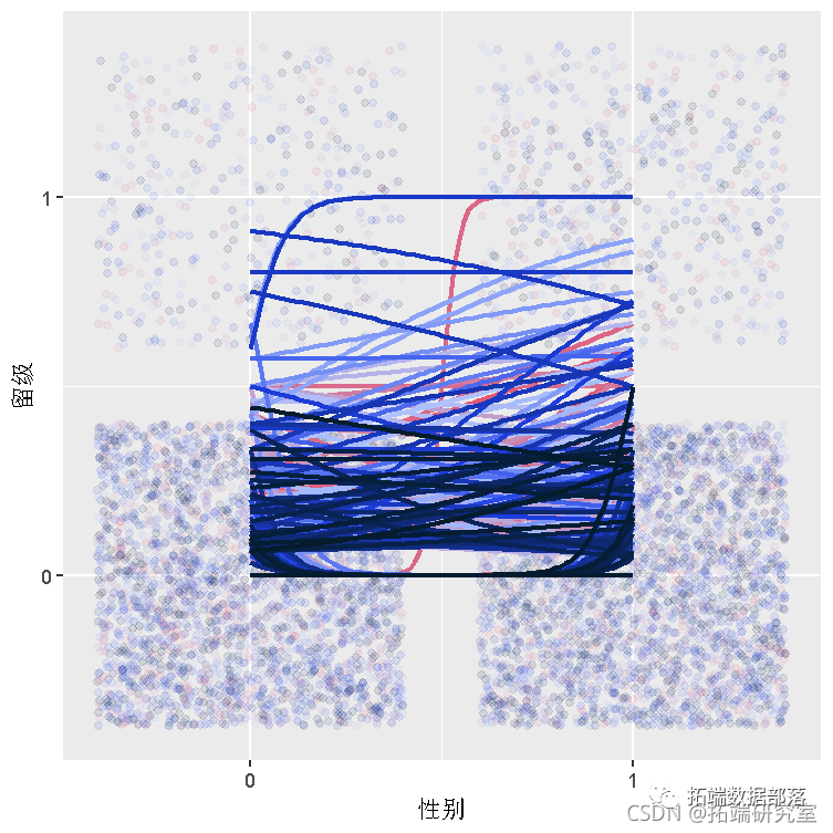
ЮвУЧгаФъСфетбљЕФСЌајБфСПЪБЃЌЮвУЧПЩвдНјааЖрЯюЪНЛиЙщ
Coefficients:Estimate Std. Error z value Pr(>|z|)(Intercept) 3.0213 0.2903 10.408 < 2e-16 ***Pclass2 -1.3603 0.2842 -4.786 1.70e-06 ***Pclass3 -2.5569 0.2853 -8.962 < 2e-16 ***Sexmale -2.6582 0.2176 -12.216 < 2e-16 ***poly(Age, 3)1 -17.7668 3.2583 -5.453 4.96e-08 ***poly(Age, 3)2 6.0044 3.0021 2.000 0.045491 *poly(Age, 3)3 -5.9181 3.0992 -1.910 0.056188 .SibSp -0.5041 0.1317 -3.828 0.000129 ***---Signif. codes: 0 ЁЎ***ЁЏ 0.001 ЁЎ**ЁЏ 0.01 ЁЎ*ЁЏ 0.05 ЁЎ.ЁЏ 0.1 ЁЎ ЁЏ 1 (Dispersion parameter for binomial family taken to be 1) Null deviance: 964.52 on 713 degrees of freedomResidual deviance: 627.55 on 706 degrees of freedomAIC: 643.55 Number of Fisher Scoring iterations: 5
ЕЋЪЧНтЪЭВЮЪ§БфЕУКмИДдгЁЃЮвУЧзЂвтЕНШ§НзЯюдкетРяКмживЊЃЌвђДЫЮвУЧНЋЪжЖЏНјааЛиЙщ
Coefficients:Estimate Std. Error z value Pr(>|z|)(Intercept) 5.616e+00 6.565e-01 8.554 < 2e-16 ***Pclass2 -1.360e+00 2.842e-01 -4.786 1.7e-06 ***Pclass3 -2.557e+00 2.853e-01 -8.962 < 2e-16 ***Sexmale -2.658e+00 2.176e-01 -12.216 < 2e-16 ***Age -1.905e-01 5.528e-02 -3.446 0.000569 ***I(Age^2) 4.290e-03 1.854e-03 2.314 0.020669 *I(Age^3) -3.520e-05 1.843e-05 -1.910 0.056188 .SibSp -5.041e-01 1.317e-01 -3.828 0.000129 ***---Signif. codes: 0 ЁЎ***ЁЏ 0.001 ЁЎ**ЁЏ 0.01 ЁЎ*ЁЏ 0.05 ЁЎ.ЁЏ 0.1 ЁЎ ЁЏ 1 (Dispersion parameter for binomial family taken to be 1) Null deviance: 964.52 on 713 degrees of freedomResidual deviance: 627.55 on 706 degrees of freedomAIC: 643.55 Number of Fisher Scoring iterations: 5
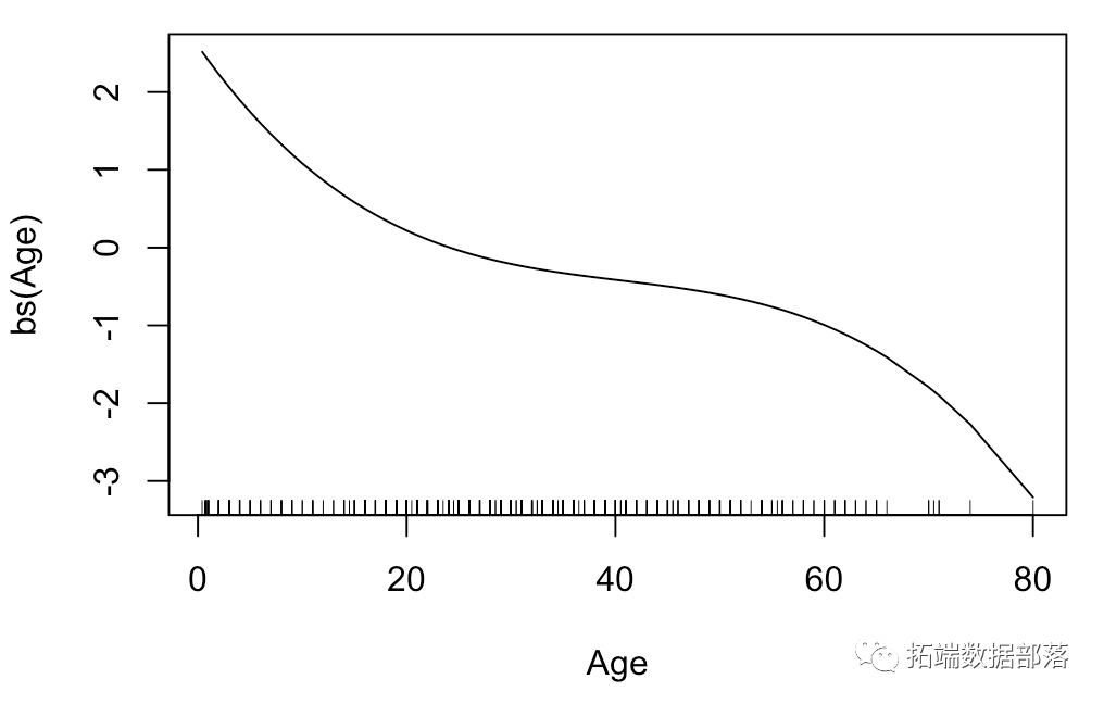
ПЩвдПДЕНЃЌpжЕЪЧЯрЭЌЕФЁЃМђЖјбджЎЃЌНЋФъСфзЊЛЛЮЊФъСфЕФЗЧЯпадКЏЪ§ЪЧгавтвхЕФЁЃПЩвдПЩЪгЛЏДЫКЏЪ§
plot(xage,yage,xlab="Age",ylab="",type="l")

ЪЕМЪЩЯЃЌЮвУЧПЩвдЪЙгУбљЬѕЧњЯпЁЃЙувхПЩМгФЃаЭЃЈ gam ЃЉЪЧЭъУРЕФПЩЪгЛЏЙЄОп
(Dispersion Parameter for binomial family taken to be 1) Null Deviance: 964.516 on 713 degrees of freedomResidual Deviance: 627.5525 on 706 degrees of freedomAIC: 643.5525177 observations deleted due to missingness Number of Local Scoring Iterations: 4 Anova for Parametric EffectsDf Sum Sq Mean Sq F value Pr(>F)Pclass 2 26.72 13.361 11.3500 1.407e-05 ***Sex 1 131.57 131.573 111.7678 < 2.2e-16 ***bs(Age) 3 22.76 7.588 6.4455 0.0002620 ***SibSp 1 14.66 14.659 12.4525 0.0004445 ***Residuals 706 831.10 1.177---Signif. codes: 0 ЁЎ***ЁЏ 0.001 ЁЎ**ЁЏ 0.01 ЁЎ*ЁЏ 0.05 ЁЎ.ЁЏ 0.1 ЁЎ ЁЏ 1
ЮвУЧПЩвдПДЕНФъСфБфСПЕФБфЛЛЃЌ
ВЂЧвЮвУЧЗЂЯжБфЛЛНгНќгкЮвУЧЕФ3НзЖрЯюЪНЁЃЮвУЧПЩвдЬэМгжУаХДјЃЌДгЖјПЩвдбщжЄИУКЏЪ§ВЛЪЧеце§ЕФЯпад

ЮвУЧЯждкгаШ§ИіФЃаЭЁЃзюКѓИјГіСЫСНИіФЃФтГЫПЭЕФдЄВтЃЌ
predict(reg,newdata=newbase,type="response")1 20.9605736 0.1368988predict(reg3,newdata=newbase,type="response")1 20.9497834 0.1218426predict(regam,newdata=newbase,type="response")1 20.9497834 0.1218426
ПЩвдПДЕНРГАКФЩЖрЁЄЕЯПЈЦеРяАТЃЈ Leonardo DiCaprioЃЉ гаДѓдМ12ЃЅЕФавДцЛњЛсЃЈПМТЧЕНЫћЕФФъСфЃЌЫћгаШ§ЕШЦБЃЌЖјЧвДЌЩЯУЛгаМвШЫЃЉЁЃ
