ЪБМфађСаФЃаЭИљОнбаОПЖдЯѓЪЧЗёЫцЛњЗжЮЊШЗЖЈадФЃаЭКЭЫцЛњадФЃаЭСНДѓРрЁЃ
ЫцЛњЪБМфађСаФЃаЭМДЪЧжИНігУЫќЕФЙ§ШЅжЕМАЫцЛњШХЖЏЯюЫљНЈСЂЦ№РДЕФФЃаЭ,НЈСЂОпЬхЕФФЃаЭ,ашНтОіШчЯТШ§ИіЮЪЬтФЃаЭЕФОпЬхаЮЪНЁЂЪБађБфСПЕФжЭКѓЦквдМАЫцЛњШХЖЏЯюЕФНсЙЙЁЃ
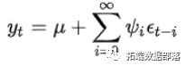
ІЬЪЧytЕФОљжЕЃЛІзЪЧЯЕЪ§ЃЌОіЖЈСЫЪБМфађСаЕФЯпадЖЏЬЌНсЙЙЃЌвВБЛГЦЮЊШЈжиЃЌЦфжаІз0=1ЃЛ{ІХt}ЮЊИпЫЙАздыЩљађСаЃЌЫќБэЪОЪБМфађСа{yt}дкtЪБПЬГіЯжСЫаТЕФаХЯЂЃЌЫљвдІХtГЦЮЊЪБПЬtЕФinnovationЃЈаТаХЯЂЃЉЛђshockЃЈШХЖЏЃЉЁЃ
ЕЅЮЛИљВтЪдЪЧЦНЮШадМьбщЕФЬиЪтЗНЗЈЁЃЕЅЮЛИљМьбщЪЧЖдЪБМфађСаНЈСЂARMAФЃаЭЁЂARIMAФЃаЭЁЂБфСПМфЕФаећЗжЮіЁЂвђЙћЙиЯЕМьбщЕШЕФЛљДЁЁЃ
ЖдгкЕЅЮЛИљВтЪдЃЌЮЊСЫЫЕУїетаЉВтЪдЕФЪЕЯжЃЌПМТЧвдЯТЯЕСа
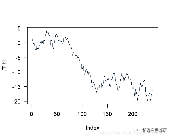
> plot(X,type="l")
- Dickey FullerЃЈБъзМЃЉ
етРяЃЌЖдгкDickey-FullerВтЪдЕФМђЕЅАцБОЃЌЮвУЧМйЩш

ЮвУЧЯыВтЪдЪЧЗёЃЈЛђВЛЪЧЃЉЁЃЮвУЧПЩвдНЋвдЧАЕФБэЪОаДЮЊ

ЫљвдЮвУЧжЛашВтЪдЯпадЛиЙщжаЕФЛиЙщЯЕЪ§ЪЧЗёЮЊПеЁЃетПЩвдЭЈЙ§бЇЩњtМьбщРДЭъГЩЁЃШчЙћЮвУЧПМТЧЧАУцЕФФЃаЭУЛгаЯпадЦЏвЦЃЌЮвУЧБиаыПМТЧЯТУцЕФЛиЙщ
Call:
lm(formula = z.diff ~ 0 + z.lag.1)
Residuals:
     Min       1Q   Median       3Q      Max
-2.84466 -0.55723 -0.00494  0.63816  2.54352
Coefficients:
         Estimate Std. Error t value Pr(>|t|)
z.lag.1 -0.005609   0.007319  -0.766    0.444
Residual standard error: 0.963 on 238 degrees of freedom
Multiple R-squared:  0.002461,    Adjusted R-squared:  -0.00173
F-statistic: 0.5873 on 1 and 238 DF,  p-value: 0.4442
ЮвУЧЕФВтЪдГЬађНЋЛљгкбЇЩњtМьбщЕФжЕЃЌ
> summary(lm(z.diff~0+z.lag.1 ))$coefficients[1,3]
[1] -0.7663308
ете§ЪЧМЦЫуЪЙгУЕФжЕ
ur.df(X,type="none",lags=0)
###############################################################
# Augmented Dickey-Fuller Test Unit Root / Cointegration Test #
###############################################################
The value of the test statistic is: -0.7663
ПЩвдЪЙгУСйНчжЕЃЈ99%ЁЂ95%ЁЂ90%ЃЉРДНтЪЭИУжЕ
> qnorm(c(.01,.05,.1)/2)
[1] -2.575829 -1.959964 -1.644854
ШчЙћЭГМЦСПГЌЙ§етаЉжЕЃЌФЧУДађСаОЭВЛЪЧЦНЮШЕФЃЌвђЮЊЮвУЧВЛФмОмОјетбљЕФМйЩшЁЃЫљвдЮвУЧПЩвдЕУГіНсТлЃЌгавЛИіЕЅЮЛИљЁЃЪЕМЪЩЯЃЌетаЉСйНчжЕЪЧЭЈЙ§
###############################################
# Augmented Dickey-Fuller Test Unit Root Test #
###############################################
Test regression none
Call:
lm(formula = z.diff ~ z.lag.1 - 1)
Residuals:
     Min       1Q   Median       3Q      Max
-2.84466 -0.55723 -0.00494  0.63816  2.54352
Coefficients:
         Estimate Std. Error t value Pr(>|t|)
z.lag.1 -0.005609   0.007319  -0.766    0.444
Residual standard error: 0.963 on 238 degrees of freedom
Multiple R-squared:  0.002461,    Adjusted R-squared:  -0.00173
F-statistic: 0.5873 on 1 and 238 DF,  p-value: 0.4442
Value of test-statistic is: -0.7663
Critical values for test statistics:
      1pct  5pct 10pct
tau1 -2.58 -1.95 -1.62
RгаМИИіАќПЩвдгУгкЕЅЮЛИљВтЪдЁЃ
Augmented Dickey-Fuller Test
data:  X
Dickey-Fuller = -2.0433, Lag order = 0, p-value = 0.5576
alternative hypothesis: stationary
етРяЛЙгавЛИіМьбщСуМйЩшЪЧДцдкЕЅЮЛИљЁЃЕЋЪЧpжЕЪЧЭъШЋВЛЭЌЕФЁЃ
p.value
[1] 0.4423705
testreg$coefficients[4]
[1] 0.4442389
- діЙуDickey-FullerМьбщ
ЛиЙщжаПЩФмгавЛаЉжЭКѓЯжЯѓЁЃР§ШчЃЌЮвУЧПЩвдПМТЧ

ЭЌбљЃЌЮвУЧашвЊМьВщвЛИіЯЕЪ§ЪЧЗёЮЊСуЁЃетПЩвдгУбЇЩњtМьбщРДзіЁЃ
> summary(lm(z.diff~0+z.lag.1+z.diff.lag ))
Call:
lm(formula = z.diff ~ 0 + z.lag.1 + z.diff.lag)
Residuals:
     Min       1Q   Median       3Q      Max
-2.87492 -0.53977 -0.00688  0.64481  2.47556
Coefficients:
            Estimate Std. Error t value Pr(>|t|)
z.lag.1    -0.005394   0.007361  -0.733    0.464
z.diff.lag -0.028972   0.065113  -0.445    0.657
Residual standard error: 0.9666 on 236 degrees of freedom
Multiple R-squared:  0.003292,    Adjusted R-squared:  -0.005155
F-statistic: 0.3898 on 2 and 236 DF,  p-value: 0.6777
coefficients[1,3]
[1] -0.7328138
ИУжЕЪЧЪЙгУ
> df=ur.df(X,type="none",lags=1)
###############################################
# Augmented Dickey-Fuller Test Unit Root Test #
###############################################
Test regression none
Call:
lm(formula = z.diff ~ z.lag.1 - 1 + z.diff.lag)
Residuals:
     Min       1Q   Median       3Q      Max
-2.87492 -0.53977 -0.00688  0.64481  2.47556
Coefficients:
            Estimate Std. Error t value Pr(>|t|)
z.lag.1    -0.005394   0.007361  -0.733    0.464
z.diff.lag -0.028972   0.065113  -0.445    0.657
Residual standard error: 0.9666 on 236 degrees of freedom
Multiple R-squared:  0.003292,    Adjusted R-squared:  -0.005155
F-statistic: 0.3898 on 2 and 236 DF,  p-value: 0.6777
Value of test-statistic is: -0.7328
Critical values for test statistics:
      1pct  5pct 10pct
tau1 -2.58 -1.95 -1.62
ЭЌбљЃЌвВПЩвдЪЙгУЦфЫћАќЃК
Augmented Dickey-Fuller Test
data:  X
Dickey-Fuller = -1.9828, Lag order = 1, p-value = 0.5831
alternative hypothesis: stationary
НсТлЪЧвЛбљЕФЃЈЮвУЧгІИУОмОјађСаЪЧЦНЮШЕФМйЩшЃЉЁЃ
- ДјЧїЪЦКЭЦЏвЦЕФдіЙуDickey-FullerМьбщ
ЕНФПЧАЮЊжЙЃЌЮвУЧЕФФЃаЭжаЛЙУЛгаАќРЈЦЏвЦЁЃЕЋКмМђЕЅЃЈетНЋБЛГЦЮЊЧАвЛЙ§ГЬЕФРЉГфАцБОЃЉЃКЮвУЧжЛашвЊдкЛиЙщжаАќКЌвЛИіГЃЪ§ЃЌ
> summary(lm) Residuals: Min 1Q Median 3Q Max -2.91930 -0.56731 -0.00548 0.62932 2.45178 Coefficients: Estimate Std. Error t value Pr(>|t|) (Intercept) 0.29175 0.13153 2.218 0.0275 * z.lag.1 -0.03559 0.01545 -2.304 0.0221 * z.diff.lag -0.01976 0.06471 -0.305 0.7603 --- Signif. codes: 0 ЁЎ***ЁЏ 0.001 ЁЎ**ЁЏ 0.01 ЁЎ*ЁЏ 0.05 ЁЎ.ЁЏ 0.1 ЁЎ ЁЏ 1 Residual standard error: 0.9586 on 235 degrees of freedom Multiple R-squared: 0.02313, Adjusted R-squared: 0.01482 F-statistic: 2.782 on 2 and 235 DF, p-value: 0.06393
ПМТЧЕНЗНВюЪфГіЕФвЛаЉЗжЮіЃЌетРяЛёЕУСЫИааЫШЄЕФЭГМЦЪ§ОнЃЌЦфжаИУФЃаЭгыУЛгаМЏГЩВПЗжЕФФЃаЭНјааСЫБШНЯЃЌвдМАЦЏвЦЃЌ
> summary(lmcoefficients[2,3]
[1] -2.303948
> anova(lm$F[2]
[1] 2.732912
етСНИіжЕвВЪЧЭЈЙ§
ur.df(X,type="drift",lags=1) ############################################### # Augmented Dickey-Fuller Test Unit Root Test # ############################################### Test regression drift Residuals: Min 1Q Median 3Q Max -2.91930 -0.56731 -0.00548 0.62932 2.45178 Coefficients: Estimate Std. Error t value Pr(>|t|) (Intercept) 0.29175 0.13153 2.218 0.0275 * z.lag.1 -0.03559 0.01545 -2.304 0.0221 * z.diff.lag -0.01976 0.06471 -0.305 0.7603 --- Signif. codes: 0 ЁЎ***ЁЏ 0.001 ЁЎ**ЁЏ 0.01 ЁЎ*ЁЏ 0.05 ЁЎ.ЁЏ 0.1 ЁЎ ЁЏ 1 Residual standard error: 0.9586 on 235 degrees of freedom Multiple R-squared: 0.02313, Adjusted R-squared: 0.01482 F-statistic: 2.782 on 2 and 235 DF, p-value: 0.06393 Value of test-statistic is: -2.3039 2.7329 Critical values for test statistics: 1pct 5pct 10pct tau2 -3.46 -2.88 -2.57 phi1 6.52 4.63 3.81
ЮвУЧЛЙПЩвдАќРЈвЛИіЯпадЧїЪЦЃЌ
> temps=(lags+1):n lm(z.diff~1+temps+z.lag.1+z.diff.lag ) Residuals: Min 1Q Median 3Q Max -2.87727 -0.58802 -0.00175 0.60359 2.47789 Coefficients: Estimate Std. Error t value Pr(>|t|) (Intercept) 0.3227245 0.1502083 2.149 0.0327 * temps -0.0004194 0.0009767 -0.429 0.6680 z.lag.1 -0.0329780 0.0166319 -1.983 0.0486 * z.diff.lag -0.0230547 0.0652767 -0.353 0.7243 --- Signif. codes: 0 ЁЎ***ЁЏ 0.001 ЁЎ**ЁЏ 0.01 ЁЎ*ЁЏ 0.05 ЁЎ.ЁЏ 0.1 ЁЎ ЁЏ 1 Residual standard error: 0.9603 on 234 degrees of freedom Multiple R-squared: 0.0239, Adjusted R-squared: 0.01139 F-statistic: 1.91 on 3 and 234 DF, p-value: 0.1287 > summary(lmcoefficients[3,3] [1] -1.98282 > anova(lm$F[2] [1] 2.737086
ЖјRКЏЪ§ЗЕЛи
ur.df(X,type="trend",lags=1) ############################################### # Augmented Dickey-Fuller Test Unit Root Test # ############################################### Test regression trend Residuals: Min 1Q Median 3Q Max -2.87727 -0.58802 -0.00175 0.60359 2.47789 Coefficients: Estimate Std. Error t value Pr(>|t|) (Intercept) 0.3227245 0.1502083 2.149 0.0327 * z.lag.1 -0.0329780 0.0166319 -1.983 0.0486 * tt -0.0004194 0.0009767 -0.429 0.6680 z.diff.lag -0.0230547 0.0652767 -0.353 0.7243 --- Signif. codes: 0 ЁЎ***ЁЏ 0.001 ЁЎ**ЁЏ 0.01 ЁЎ*ЁЏ 0.05 ЁЎ.ЁЏ 0.1 ЁЎ ЁЏ 1 Residual standard error: 0.9603 on 234 degrees of freedom Multiple R-squared: 0.0239, Adjusted R-squared: 0.01139 F-statistic: 1.91 on 3 and 234 DF, p-value: 0.1287 Value of test-statistic is: -1.9828 1.8771 2.7371 Critical values for test statistics: 1pct 5pct 10pct tau3 -3.99 -3.43 -3.13 phi2 6.22 4.75 4.07 phi3 8.43 6.49 5.47
- KPSS Мьбщ
дкетРяЃЌдкKPSSЙ§ГЬжаЃЌПЩвдПМТЧСНжжФЃаЭЃКЦЏвЦФЃаЭЛђЯпадЧїЪЦФЃаЭЁЃдкетРяЃЌСуМйЩшЪЧађСаЪЧЦНЮШЕФЁЃ
ДњТыЪЧ
ur.kpss(X,type="mu")
#######################
# KPSS Unit Root Test #
#######################
Test is of type: mu with 4 lags.
Value of test-statistic is: 0.972
Critical value for a significance level of:
                10pct  5pct 2.5pct  1pct
critical values 0.347 0.463  0.574 0.73
дкетжжЧщПіЯТЃЌгавЛжжЧїЪЦ
ur.kpss(X,type="tau")
#######################
# KPSS Unit Root Test #
#######################
Test is of type: tau with 4 lags.
Value of test-statistic is: 0.5057
Critical value for a significance level of:
                10pct  5pct 2.5pct  1pct
critical values 0.119 0.146  0.176 0.216
дйвЛДЮЃЌПЩвдЪЙгУСэвЛИіАќРДЛёЕУЯрЭЌЕФМьбщЃЈЕЋЭЌбљЃЌВЛЭЌЕФЪфГіЃЉ
KPSS Test for Level Stationarity
data:  X
KPSS Level = 1.1997, Truncation lag parameter = 3, p-value = 0.01
> kpss.test(X,"Trend")
    KPSS Test for Trend Stationarity
data:  X
KPSS Trend = 0.6234, Truncation lag parameter = 3, p-value = 0.01
жСЩйгавЛжТадЃЌвђЮЊЮвУЧвЛжБОмОјМйЩшЁЃ
- Philipps-Perron Мьбщ
Philipps-PerronМьбщЛљгкADFЙ§ГЬЁЃДњТы
> PP.test(X)
    Phillips-Perron Unit Root Test
data:  X
Dickey-Fuller = -2.0116, Truncation lag parameter = 4, p-value = 0.571
СэвЛжжПЩФмЕФЬцДњЗНАИЪЧ
> pp.test(X)
    Phillips-Perron Unit Root Test
data:  X
Dickey-Fuller Z(alpha) = -7.7345, Truncation lag parameter = 4, p-value
= 0.6757
alternative hypothesis: stationary
- БШНЯ
ЮвВЛЛсЛЈИќЖрЕФЪБМфБШНЯВЛЭЌЕФДњТыЃЌдкRжаЃЌдЫааетаЉВтЪдЁЃЮвУЧдйЛЈЕуЪБМфПьЫйБШНЯвЛЯТетШ§жжЗНЗЈЁЃШУЮвУЧЩњГЩвЛаЉЛђЖрЛђЩйОпгаздЯрЙиЕФздЛиЙщЙ§ГЬЃЌвдМАвЛаЉЫцЛњгЮзпЃЌШУЮвУЧПДПДетаЉМьбщЪЧШчКЮжДааЕФЃК
> for(i in 1:(length(AR)+1)
+ for(s in 1:1000){
+ if(i!=1) X=arima.sim
+ M2[s,i]=(pp.testp.value)
+ M1[s,i]=(kpss.testp.value)
+ M3[s,i]=(adf.testp.value)
+ }
етРяЃЌЮвУЧвЊМЦЫуМьбщЕФpжЕГЌЙ§5%ЕФДЮЪ§ЃЌ
> plot(AR,P[1,],type="l",col="red",ylim=c(0,1)
> lines(AR,P[2,],type="l",col="blue")
> lines(AR,P[3,],type="l",col="green")
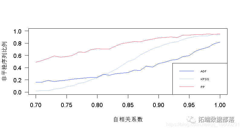
ЮвУЧПЩвддкетРяПДЕНDickey-FullerВтЪдЕФБэЯжгаЖрВЛЮШЖЈЃЌвђЮЊЮвУЧЕФздЛиЙщЙ§ГЬжага50%(жСЩй)БЛШЯЮЊЪЧЗЧЦНЮШЕФЁЃ