зюНќЮвБЛвЊЧѓзЋаДЙигкН№ШкЪБМфађСаЕФcopulasЕФЕїВщЁЃДгЖСШЁЪ§ОнжаЛёЕУИїжжФЃаЭЕФУшЪіЃЌАќРЈвЛаЉЭМаЮКЭЭГМЦЪфГіЁЃ
> oil = read.xlsxЃЈtempЃЌsheetName =ЁАDATAЁБЃЌdec =ЁАЃЌЁБЃЉ
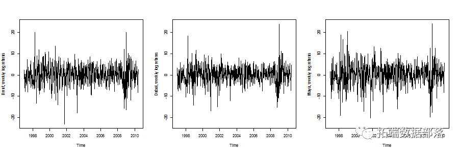
ШЛКѓЮвУЧПЩвдЛцжЦетШ§ИіЪБМфађСа
1 1997-01-10 2.73672 2.25465 3.3673 1.5400


2 1997-01-17 -3.40326 -6.01433 -3.8249 -4.1076


3 1997-01-24 -4.09531 -1.43076 -6.6375 -4.6166


4 1997-01-31 -0.65789 0.34873 0.7326 -1.5122


5 1997-02-07 -3.14293 -1.97765 -0.7326 -1.8798


6 1997-02-14 -5.60321 -7.84534 -7.6372 -11.0549
етИіЯыЗЈЪЧдкетРяЪЙгУвЛаЉЖрБфСПARMA-GARCHЙ§ГЬЁЃетРяЕФЦєЗЂЪНЪЧЕквЛВПЗжгУгкФЃФтЪБМфађСаЦНОљжЕЕФЖЏЬЌЃЌЕкЖўВПЗжгУгкФЃФтЪБМфађСаЗНВюЕФЖЏЬЌЁЃ
БОЮФПМТЧСЫСНжжФЃаЭ
- ЙигкARMAФЃаЭВаВюЕФЖрБфСПGARCHЙ§ГЬЃЈЛђЗНВюОиеѓЖЏСІбЇФЃаЭЃЉ
- ЙигкARMA-GARCHЙ§ГЬВаВюЕФЖрБфСПФЃаЭЃЈЛљгкcopulaЃЉ
вђДЫЃЌетРяНЋПМТЧВЛЭЌЕФађСаЃЌзїЮЊВЛЭЌФЃаЭЕФВаВюЛёЕУЁЃЮвУЧЛЙПЩвдНЋетаЉВаВюБъзМЛЏЁЃ
ARMAФЃаЭ
> fit1 = arimaЃЈx = dat [ЃЌ1]ЃЌorder = cЃЈ2,0,1ЃЉЃЉ > fit2 = arimaЃЈx = dat [ЃЌ2]ЃЌorder = cЃЈ1,0,1ЃЉЃЉ > fit3 = arimaЃЈx = dat [ЃЌ3]ЃЌorder = cЃЈ1,0,1ЃЉЃЉ > m < - applyЃЈdat_armaЃЌ2ЃЌmeanЃЉ > v < - applyЃЈdat_armaЃЌ2ЃЌvarЃЉ > dat_arma_std < - tЃЈЃЈtЃЈdat_armaЃЉ-mЃЉ/ sqrtЃЈvЃЉЃЉ
ARMA-GARCHФЃаЭ
> fit1 = garchFitЃЈformula = ~armaЃЈ2,1ЃЉ+ garchЃЈ1,1ЃЉЃЌdata = dat [ЃЌ1]ЃЌcond.dist =ЁАstdЁБЃЉ > fit2 = garchFitЃЈformula = ~armaЃЈ1,1ЃЉ+ garchЃЈ1,1ЃЉЃЌdata = dat [ЃЌ2]ЃЌcond.dist =ЁАstdЁБЃЉ > fit3 = garchFitЃЈformula = ~armaЃЈ1,1ЃЉ+ garchЃЈ1,1ЃЉЃЌdata = dat [ЃЌ3]ЃЌcond.dist =ЁАstdЁБЃЉ > m_res < - applyЃЈdat_resЃЌ2ЃЌmeanЃЉ > v_res < - applyЃЈdat_resЃЌ2ЃЌvarЃЉ > dat_res_std = cbindЃЈЃЈdat_res [ЃЌ1] -m_res [1]ЃЉ/ sqrtЃЈv_res [1]ЃЉЃЌЃЈdat_res [ЃЌ2] -m_res [2]ЃЉ/ sqrtЃЈv_res [2]ЃЉЃЌЃЈdat_res [ ЃЌ3] -m_res [3]ЃЉ/ SQRTЃЈv_res [3]ЃЉЃЉ
ЖрБфСПGARCHФЃаЭ
ПЩвдПМТЧЕФЕквЛИіФЃаЭЪЧаЗНВюОиеѓЕФЖрБфСПEWMAЃЌ
> ewma = EWMAvolЃЈdat_res_stdЃЌlambda = 0.96ЃЉ
ВЈЖЏад
> emwa_series_vol = functionЃЈi = 1ЃЉ{ + linesЃЈTimeЃЌdat_arma [ЃЌi] + 40ЃЌcol =ЁАgrayЁБЃЉ + j = 1 + ifЃЈi == 2ЃЉj = 5 + ifЃЈi == 3ЃЉj = 9

вўКЌЯрЙиад
> emwa_series_cor = functionЃЈi = 1ЃЌj = 2ЃЉ{ + ifЃЈЃЈminЃЈiЃЌjЃЉ== 1ЃЉЃІЃЈmaxЃЈiЃЌjЃЉ== 2ЃЉЃЉ{ + a = 1; B = 9; AB = 3} + r = ewma $ Sigma.t [ЃЌab] / sqrtЃЈewma $ Sigma.t [ЃЌa] * + ewma $ Sigma.t [ЃЌb]ЃЉ + plotЃЈTimeЃЌrЃЌtype =ЁАlЁБЃЌylim = cЃЈ0,1ЃЉЃЉ +}

ЖрБфСПGARCHЃЌМДBEKKЃЈ1,1ЃЉФЃаЭЃЌР§ШчЪЙгУЃК
> bekk = BEKK11ЃЈdat_armaЃЉ > bekk_series_vol functionЃЈi = 1ЃЉ{ + plotЃЈTimeЃЌ $ Sigma.t [ЃЌ1]ЃЌtype =ЁАlЁБЃЌ + ylab = ЃЈdatЃЉ[i]ЃЌcol =ЁАwhiteЁБЃЌylim = cЃЈ0,80ЃЉЃЉ + linesЃЈTimeЃЌdat_arma [ЃЌi] + 40ЃЌcol =ЁАgrayЁБЃЉ + j = 1 + ifЃЈi == 2ЃЉj = 5 + ifЃЈi == 3ЃЉj = 9 > bekk_series_cor = functionЃЈi = 1ЃЌj = 2ЃЉ{ + a = 1; B = 5; AB = 2} + a = 1; B = 9; AB = 3} + a = 5; B = 9; AB = 6} + r = bk $ Sigma.t [ЃЌab] / sqrtЃЈbk $ Sigma.t [ЃЌa] * + bk $ Sigma.t [ЃЌb]ЃЉ

ДгЕЅБфСПGARCHФЃаЭжаФЃФтВаВю
ЕквЛВНПЩФмЪЧПМТЧВаВюЕФвЛаЉОВЬЌЃЈСЊКЯЃЉЗжВМЁЃЕЅБфСПБпдЕЗжВМЪЧ

БпдЕУмЖШЕФТжРЊЃЈЪЙгУЫЋБфСПКЫЙРМЦЛёЕУЃЉ

вВПЩвдНЋcopulaУмЖШПЩЪгЛЏЃЈЩЯУцгавЛаЉЗЧВЮЪ§ЙРМЦЃЌЯТУцЪЧВЮЪ§copulaЃЉ
> copula_NP = functionЃЈi = 1ЃЌj = 2ЃЉ{ + n = nrowЃЈuvЃЉ + s = 0.3 + norm.cop < - normalCopulaЃЈ0.5ЃЉ + norm.cop < - normalCopulaЃЈfitCopulaЃЈnorm.copЃЌuvЃЉ@estimateЃЉ + dc = functionЃЈxЃЌyЃЉdCopulaЃЈcbindЃЈxЃЌyЃЉЃЌnorm.copЃЉ + ylab = namesЃЈdatЃЉ[j]ЃЌzlab =ЁАcopule GaussienneЁБЃЌticktype =ЁАdetailedЁБЃЌzlim = zlЃЉ + + t.cop < - tCopulaЃЈ0.5ЃЌdf = 3ЃЉ + t.cop < - tCopulaЃЈt.fit [1]ЃЌdf = t.fit [2]ЃЉ + ylab = namesЃЈdatЃЉ[j]ЃЌzlab =ЁАcopule de StudentЁБЃЌticktype =ЁАdetailedЁБЃЌzlim = zlЃЉ +}

ПЩвдПМТЧетИі  КЏЪ§ЃЌ

МЦЫуШ§ИіађСаЕФЕФОбщАцБОЃЌВЂНЋЦфгывЛаЉВЮЪ§АцБОНјааБШНЯЃЌ
> > lambda = functionЃЈCЃЉ{ + l = functionЃЈuЃЉpcopulaЃЈCЃЌcbindЃЈuЃЌuЃЉЃЉ/ u + v = VectorizeЃЈlЃЉЃЈuЃЉ + returnЃЈcЃЈvЃЌrevЃЈvЃЉЃЉЃЉ +} > > graph_lambda = functionЃЈiЃЌjЃЉ{ + X = dat_res + U = rankЃЈX [ЃЌi]ЃЉ/ЃЈnrowЃЈXЃЉ+1ЃЉ + V = rankЃЈX [ЃЌj]ЃЉ/ЃЈnrowЃЈXЃЉ+1ЃЉ + normal.cop < - normalCopulaЃЈ.5ЃЌdim = 2ЃЉ + t.cop < - tCopulaЃЈ.5ЃЌdim = 2ЃЌdf = 3ЃЉ + fit1 = fitCopulaЃЈnormal.copЃЌcbindЃЈUЃЌVЃЉЃЌmethod =ЁАmlЁБЃЉ dЃЈUЃЌVЃЉЃЌmethod =ЁАmlЁБЃЉ + C1 = normalCopulaЃЈfit1 @ copula @ parametersЃЌdim = 2ЃЉ + C2 = tCopulaЃЈfit2 @ copula @ parameters [1]ЃЌdim = 2ЃЌdf = truncЃЈfit2 @ copula @ parameters [2]ЃЉЃЉ +

ЕЋШЫУЧПЩФмЯыжЊЕРЯрЙиадЪЧЗёЫцЪБМфЮШЖЈЁЃ
> time_varying_correl_2 = functionЃЈi = 1ЃЌj = 2ЃЌ + nom_arg =ЁАPearsonЁБЃЉ{ + uv = dat_arma [ЃЌcЃЈiЃЌjЃЉ] nom_argЃЉЃЉ[1,2] +} > time_varying_correl_2ЃЈ1,2ЃЉ > time_varying_correl_2ЃЈ1,2ЃЌЁАspearmanЁБЃЉ > time_varying_correl_2ЃЈ1,2ЃЌЁАkendallЁБЃЉ

ЫЙЦЄЖћТќгыЪББфХХУћЯрЙиЯЕЪ§

ЛђПЯЕТЖћ ЯрЙиЯЕЪ§

ЮЊСЫФЃаЭЕФЯрЙиадЃЌПМТЧDCCФЃаЭЃЈSЃЉ
> m2 = dccFitЃЈdat_res_stdЃЉ > m3 = dccFitЃЈdat_res_stdЃЌtype =ЁАEngleЁБЃЉ > R2 = m2 $ rho.t > R3 = m3 $ rho.t

вЊЛёЕУвЛаЉдЄВтЃЌ ЪЙгУР§Шч
> garch11.spec = ugarchspecЃЈmean.model = listЃЈarmaOrder = cЃЈ2,1ЃЉЃЉЃЌvariance.model = listЃЈgarchOrder = cЃЈ1,1ЃЉЃЌmodel =ЁАGARCHЁБЃЉЃЉ > dcc.garch11.spec = dccspecЃЈuspec = multispecЃЈreplicateЃЈ3ЃЌgarch11.specЃЉЃЉЃЌdccOrder = cЃЈ1,1ЃЉЃЌ distribution =ЁАmvnormЁБЃЉ > dcc.fit = dccfitЃЈdcc.garch11.specЃЌdata = datЃЉ > fcst = dccforecastЃЈdcc.fitЃЌn.ahead = 200ЃЉ

