ФПТМ
дѕУДзіВтЪд
аЗНВюЗжЮі
ФтКЯЯпЕФМђЕЅЭМНт
ФЃаЭЕФpжЕКЭRЦНЗН
МьВщФЃаЭЕФМйЩш
ОпгаШ§РрКЭIIаЭЦНЗНКЭЕФаЗНВюЪОР§ЗжЮі
аЗНВюЗжЮі
ФтКЯЯпЕФМђЕЅЭМНт
зщКЯФЃаЭЕФpжЕКЭRЦНЗН
МьВщФЃаЭЕФМйЩш
дѕУДзіВтЪд
ОпгаСНИіРрБ№КЭIIаЭЦНЗНКЭЕФаЗНВюЪОР§ЕФЗжЮі
БОЪОР§ЪЙгУIIаЭЦНЗНКЭ ЁЃВЮЪ§ЙРМЦжЕдкRжаЕФМЦЫуЗНЪНВЛЭЌЃЌ
Data = read.table(textConnection(Input),header=TRUE)


 plot(x   = Data$Temp,
     y   = Data$Pulse,
     col = Data$Species,
     pch = 16,
     xlab = "Temperature",
     ylab = "Pulse")

legend('bottomright',
       legend = levels(Data$Species),
       col = 1:2,
       cex = 1,
       pch = 16)
аЗНВюЗжЮі
Anova Table (Type II tests)


             Sum Sq Df  F value    Pr(>F)

Temp         4376.1  1 1388.839 < 2.2e-16 ***

Species       598.0  1  189.789 9.907e-14 ***

Temp:Species    4.3  1    1.357    0.2542


### Interaction is not significant, so the slope across groups

### is not different.


model.2 = lm (Pulse ~ Temp + Species,
              data = Data)

library(car)

Anova(model.2, type="II")


Anova Table (Type II tests)


          Sum Sq Df F value    Pr(>F)

Temp      4376.1  1  1371.4 < 2.2e-16 ***

Species    598.0  1   187.4 6.272e-14 ***


### The category variable (Species) is significant,

### so the intercepts among groups are different


Coefficients:

             Estimate Std. Error t value Pr(>|t|)

(Intercept)  -7.21091    2.55094  -2.827  0.00858 **

Temp          3.60275    0.09729  37.032  < 2e-16 ***

Speciesniv  -10.06529    0.73526 -13.689 6.27e-14 ***


###   but the calculated results will be identical.

### The slope estimate is the same.

### The intercept for species 1 (ex) is (intercept).

### The intercept for species 2 (niv) is (intercept) + Speciesniv.

### This is determined from the contrast coding of the Species

### variable shown below, and the fact that Speciesniv is shown in

### coefficient table above.


    niv

ex    0

niv   1
ФтКЯЯпЕФМђЕЅЭМНт
plot(x   = Data$Temp,
     y   = Data$Pulse,
     col = Data$Species,
     pch = 16,
     xlab = "Temperature",
     ylab = "Pulse")
ФЃаЭЕФpжЕКЭRЦНЗН
Multiple R-squared:  0.9896,  Adjusted R-squared:  0.9888

F-statistic:  1331 on 2 and 28 DF,  p-value: < 2.2e-16
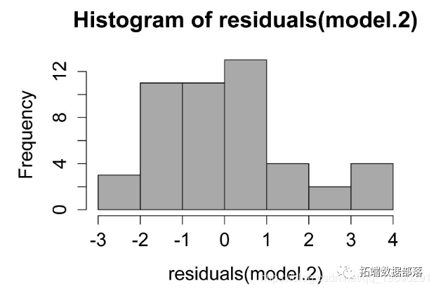
МьВщФЃаЭЕФМйЩш
ЯпадФЃаЭжаВаВюЕФжБЗНЭМЁЃетаЉВаВюЕФЗжВМгІНќЫЦе§ЬЌЁЃ

ВаВюгыдЄВтжЕЕФЙиЯЕЭМЁЃВаВюгІЮоЦЋЧвОљЕШЁЃ
### additional model checking plots with: plot(model.2)
### alternative: library(FSA); residPlot(model.2)
ОпгаШ§РрКЭIIаЭЦНЗНКЭЕФаЗНВюЪОР§ЗжЮі
БОЪОР§ЪЙгУIIаЭЦНЗНКЭЃЌВЂПМТЧОпгаШ§ИізщЕФЧщПіЁЃ
### --------------------------------------------------------------
### Analysis of covariance, hypothetical data
### --------------------------------------------------------------


Data = read.table(textConnection(Input),header=TRUE)


plot(x   = Data$Temp,
     y   = Data$Pulse,
     col = Data$Species,
     pch = 16,
     xlab = "Temperature",
     ylab = "Pulse")

legend('bottomright',
       legend = levels(Data$Species),
       col = 1:3,
       cex = 1,
       pch = 16)
аЗНВюЗжЮі
options(contrasts = c("contr.treatment", "contr.poly"))

   ### These are the default contrasts in R


Anova(model.1, type="II")


             Sum Sq Df   F value Pr(>F)

Temp         7026.0  1 2452.4187 <2e-16 ***

Species      7835.7  2 1367.5377 <2e-16 ***

Temp:Species    5.2  2    0.9126 0.4093


### Interaction is not significant, so the slope among groups

### is not different.


Anova(model.2, type="II")


          Sum Sq Df F value    Pr(>F)

Temp      7026.0  1  2462.2 < 2.2e-16 ***

Species   7835.7  2  1373.0 < 2.2e-16 ***

Residuals  125.6 44


### The category variable (Species) is significant,

### so the intercepts among groups are different


summary(model.2)


Coefficients:

             Estimate Std. Error t value Pr(>|t|)

(Intercept)  -6.35729    1.90713  -3.333  0.00175 **

Temp          3.56961    0.07194  49.621  < 2e-16 ***

Speciesfake  19.81429    0.66333  29.871  < 2e-16 ***

Speciesniv  -10.18571    0.66333 -15.355  < 2e-16 ***


### The slope estimate is the Temp coefficient.

### The intercept for species 1 (ex) is (intercept).

### The intercept for species 2 (fake) is (intercept) + Speciesfake.

### The intercept for species 3 (niv) is (intercept) + Speciesniv.

### This is determined from the contrast coding of the Species

### variable shown below.


contrasts(Data$Species)


     fake niv

ex      0   0

fake    1   0

niv     0   1
ФтКЯЯпЕФМђЕЅЭМНт

зщКЯФЃаЭЕФpжЕКЭRЦНЗН
Multiple R-squared:  0.9919,  Adjusted R-squared:  0.9913

F-statistic:  1791 on 3 and 44 DF,  p-value: < 2.2e-16
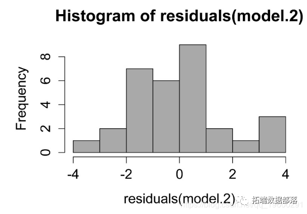
МьВщФЃаЭЕФМйЩш
hist(residuals(model.2),
col="darkgray")
ЯпадФЃаЭжаВаВюЕФжБЗНЭМЁЃетаЉВаВюЕФЗжВМгІНќЫЦе§ЬЌЁЃ
plot(fitted(model.2),
residuals(model.2))

ВаВюгыдЄВтжЕЕФЙиЯЕЭМЁЃВаВюгІЮоЦЋЧвОљЕШЁЃ
### additional model checking plots with: plot(model.2)
### alternative: library(FSA); residPlot(model.2)
